1
2
3
4
5
6
7
8
9
10
11
12
13
14
15
16
17
18
19
20
21
22
23
24
25
26
27
28
29
30
31
32
33
34
35
36
37
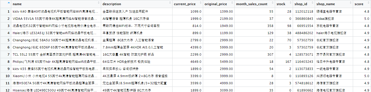
| library(readxl)
tm <- read_excel("data/tianmaoTV.xlsx", skip=1)
typeof(tm["current_price"])
typeof(tm$current_price)
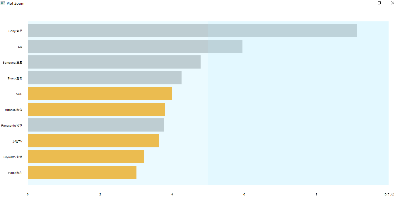
price_brands = aggregate(tm["current_price"], by=list(brand=tm$brand), mean)
price_brands$current_price
price_brands <- price_brands[order(price_brands$current_price, decreasing = T), ][1:10,]
price_brands
price_brands$brand
china <- c("AOC", "Hisense/海信", "乐视TV", "Skyworth/创维", "Haier/海尔")
price_brands$china <- ifelse(price_brands$brand%in%china, 1, 0)
price_brands
par()$mar
par(mar=c(5, 5, 2, 2))
price_brands <- price_brands[order(price_brands$current_price),]
x <- barplot(price_brands$current_price, names.arg = price_brands$brand,
horiz = T, las=1,
cex.names = 0.6,
border = NA,
col = "grey",
axes = F,
xlim = c(0, 10000))
china_price_vector <- price_brands$current_price * price_brands$china
china_price_vector
barplot(china_price_vector, names.arg = F,
horiz = T, las=1,
border = NA,
col = "orange1",
axes = F,
add = T)
axis(side = 1, at = c(0, 2000, 4000, 6000, 8000, 10000),
labels = c(0, 2, 4, 6, 8, '10(千元)'),
tick = F, cex.axis = 0.6)
rect(0, -0.5, 5000, x[10] + x[1], col = rgb(191, 239, 255, 80, maxColorValue = 255), border = NA)
rect(5000, -0.5, 10000, x[10] + x[1], col = rgb(191, 239, 255, 110, maxColorValue = 255), border = NA)
|
 ...
...